9.3 Statistical Inference for Two Population Means with Unknown Population Standard Deviations

The comparison of two population means is very common. Often, we want to find out if the two populations under study have the same mean or if there is some difference in the two population means. The approach we take when studying two population means depends on whether the samples are independent or matched. In the case the samples are independent, we also have to contend with whether or not we know the population standard deviations.

Two populations are independent if the sample taken from population 1 is not related in anyway to the sample taken from population 2. In this situation, any relationship between the samples or populations is entirely coincidental.

Throughout this section, we will use subscripts to identify the values for the means, sample sizes, and standard deviations for the two populations:

In order to construct a confidence interval or conduct a hypothesis test on the difference in two population means ([latex]\mu_1-\mu_2[/latex]), we need to use the distribution of the difference in the sample means [latex]\overline_1-\overline_2[/latex]:

• The mean of the distribution of the difference in the sample means is [latex]\displaystyle<\mu_<\overline_1-\overline_2>>=\mu_1-\mu_2[/latex].
• The standard deviation of the distribution of the difference in the sample means is [latex]\displaystyle<\sigma_<\overline_1-\overline_2>=\sqrt+\frac>>[/latex].
• The distribution of the difference in the sample means is normal if one of the following is true:
  • Both populations are normally distributed.
  • The sample sizes are large enough ([latex]n_1 \geq 30[/latex] and [latex]n_2 \geq 30[/latex]).

  As we have seen previously when working with confidence intervals and hypothesis testing for a single population, when the population standard deviation is unknown and we must use the sample standard deviation as an estimate for the population standard deviation, we use a [latex]t[/latex]-distribution. We do the same thing when working with the two population means. When the population standard deviations are unknown, we use the sample standard deviations as estimates for the population standard deviations [latex]\sigma_1[/latex] and [latex]\sigma_2[/latex]. In this situation, we use a [latex]t[/latex]-distribution for the distribution of the difference in the sample means. So, when the population standard deviations are unknown for a confidence interval or hypothesis test on the difference in two population means, we will use a [latex]t[/latex]-distribution. The [latex]t[/latex]-score and the degrees of freedom are:

  Obviously, the degrees of freedom formula is somewhat complicated. But a computer makes the calculation a bit more manageable. The output from the degrees of freedom formula is rarely a whole number. After calculating the value of [latex]df[/latex] using the above formula, round the output from this formula down to the next whole number to get the degrees of freedom for the [latex]t[/latex]-distribution.

  Constructing a Confidence Interval for the Difference in Two Population Means with Unknown Population Standard Deviations

  Suppose a sample of size [latex]n_1[/latex] with sample mean [latex]\overline_1[/latex] and standard deviation [latex]s_1[/latex] is taken from population 1 and a sample of size [latex]n_2[/latex] with sample mean [latex]\overline_2[/latex] and standard deviation [latex]s_2[/latex] is taken from population 2 where the populations are independent and the population standard deviations are unknown. The limits for the confidence interval with confidence level [latex]C[/latex] for the difference in the population means [latex]\displaystyle<\mu_1-\mu_2>[/latex] are:

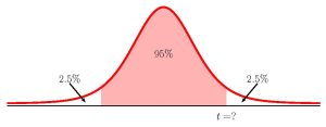
  where [latex]t[/latex] is the positive [latex]t[/latex]-score of the [latex]t[/latex]-distribution with [latex]\displaystyle+\frac\right)^2> \times \left(\frac\right)^2+\frac \times \left(\frac\right)^2>>[/latex] so that the area under the curve in between [latex]-t[/latex] and [latex]t[/latex] is [latex]C\%[/latex].

  NOTES

  1. In order to construct the confidence interval for the difference in two population means with independent samples, we need to check that the distribution of the difference in the sample means follows a normal distribution. This means that we need to check that either the populations are normal or that the sample sizes are large enough (greater than or equal to 30).
  2. When the population standard deviations are unknown, we must use a [latex]t[/latex]-distribution in the construction of the confidence interval.
  3. The value of degrees of freedom must be a whole number. After using the formula, remember to round the value down to the next whole number to get the required degrees of freedom for the [latex]t[/latex]-distribution.

  CALCULATING THE [latex]\textcolort[/latex]-SCORE FOR A CONFIDENCE INTERVAL IN EXCEL

  To find the [latex]t[/latex]-score to construct a confidence interval with confidence level [latex]C[/latex], use the t.inv.2t(area in the tails, degrees of freedom) function.

  • For area in the tails, enter the sum of the area in the tails of the [latex]t[/latex]-distribution. For a confidence interval, the area in the tails is [latex]1-C[/latex].
  • For degrees of freedom, enter the degrees of freedom calculated using [latex]\displaystyle+\frac\right)^2>\times \left(\frac\right)^2+\frac\times \left(\frac\right)^2>>[/latex].

  The output from the t.inv.2t function is the value of [latex]t[/latex]-score needed to construct the confidence interval.

  NOTE

  1. The t.inv.2t function requires that we enter the sum of the area in both tails. The area in the middle of the distribution is the confidence level [latex]C[/latex], so the sum of the area in both tails is the leftover area [latex]1-C[/latex].
  2. The degrees of freedom for a [latex]t[/latex]-distribution must be a whole number. The output from the degrees of freedom formula [latex]\displaystyle+\frac\right)^2>\times \left(\frac\right)^2+\frac\times \left(\frac\right)^2>>[/latex] is almost never a whole number. After calculating the value of [latex]df[/latex] using the formula, round the value down to the next whole number. Remember to entered the rounded down value of [latex]df[/latex] for the degrees of freedom in the t.inv.2t function.

  EXAMPLE

  A company that manufacturers and services photocopiers wants to study the difference in the average repair time for the two different models of photocopiers they make. In a sample of 60 repairs of photocopier A, the mean repair time was 84.2 minutes with a standard deviation of 19.4 minutes. In a sample of 70 repairs of photocopier B, the mean repair time was 91.6 minutes with a standard deviation of 18.8 minutes.

  1. Construct a 95% confidence interval for the difference in the mean repair time for the two photocopiers.
  2. Interpret the confidence interval found in part 1.
  3. Is there evidence to suggest that the mean repair times for the photocopiers is the same? Explain.

  Solution:

  Let photocopier A be population 1 and photocopier B be population 2. These populations are independent because there is no relationship between the repair times for the two photocopiers. From the question we have the following information:
  

  Photocopier A	Photocopier B
  [latex]n_1=60[/latex]	[latex]n_2=70[/latex]
  [latex]\overline_1=84.2[/latex]	[latex]\overline_2=91.6[/latex]
  [latex]s_1=19.4[/latex]	[latex]s_2=18.8[/latex]

  

  To find the confidence interval, we need to find the [latex]t[/latex]-score for the 95% confidence interval. This means that we need to find the [latex]t[/latex]-score so that the area in the tails is [latex]1-0.95=0.05[/latex]. [latex]\begin \\ df & = & \frac<\left(\frac+\frac\right)^2> \times \left(\frac\right)^2+\frac \times \left(\frac\right)^2> \\ & = & \frac<\left(\frac+\frac\right)^2> \times \left(\frac\right)^2+\frac \times \left(\frac\right)^2> \\ & = & 123.68. \\ & \Rightarrow & 123 \\ \\ \end[/latex]

  Function	t.inv.2t	Answer
  Field 1	0.05	1.9794…
  Field 2	123

  NOTES

  1. When calculating the limits for the confidence interval keep all of the decimals in the [latex]t[/latex]-score and other values throughout the calculation. This will ensure that there is no round-off error in the answers. You can use Excel to do the calculation of the limits, clicking on the cells containing the [latex]t[/latex]-score and any other values, to ensure that all of the decimal places are used in the calculation.
  2. When writing down the interpretation of the confidence interval, make sure to include the confidence level, the actual difference in the population means captured by the confidence interval (i.e. be specific to the context of the question), and appropriate units for the limits.
  3. The value of the degrees of freedom must be a whole number. After using the formula, remember to round the value down to the next whole number to get the required degrees of freedom for the [latex]t[/latex]-distribution.

  Steps to Conduct a Hypothesis Test for the Difference in Two Independent Population Means with Unknown Population Standard Deviations

  1. Write down the null hypothesis that there is no difference in the population means: [latex]\begin \\ H_0: & & \mu_1-\mu_2=0 \\ \end[/latex] The null hypothesis is always the claim that the two population means are equal ([latex]\mu_1=\mu_2[/latex]).
  2. Write down the alternative hypotheses in terms of the difference in the population means. The alternative hypothesis will be one of the following: [latex]\begin \\ H_a: \mu_1-\mu_2 0 & & (\mu_1 \gt \mu_2) \\ H_a: \mu_1-\mu_2 \neq 0 & & (\mu_1 \neq \mu_2) \\ \\ \end[/latex]
  3. Use the form of the alternative hypothesis to determine if the test is left-tailed, right-tailed, or two-tailed.
  4. Collect the sample information for the test and identify the significance level.
  5. Assuming the population standard deviations are unknown, use a [latex]t[/latex]-distribution to find the p-value (the area in the corresponding tail) for the test. The [latex]t[/latex]-score and degrees of freedom are [latex]\begin t & = & \frac<(\overline_1-\overline_2)-(\mu_1-\mu_2)>+\frac>> \\ \\ df & = & \frac<\left(\frac+\frac\right)^2>\times \left(\frac\right)^2+\frac\times \left(\frac\right)^2> \\ \\ \end[/latex]
  6. Compare the p-value to the significance level and state the outcome of the test:
     • If p-value[latex]\leq \alpha[/latex], reject [latex]H_0[/latex] in favour of [latex]H_a[/latex].
       • The results of the sample data are significant. There is sufficient evidence to conclude that the null hypothesis [latex]H_0[/latex] is an incorrect belief and that the alternative hypothesis [latex]H_a[/latex] is most likely correct.
     • If p-value[latex]\gt \alpha[/latex], do not reject [latex]H_0[/latex].
       • The results of the sample data are not significant. There is not sufficient evidence to conclude that the alternative hypothesis [latex]H_a[/latex] may be correct.
  7. Write down a concluding sentence specific to the context of the question.

  USING EXCEL TO CALCULE THE P-VALUE FOR A HYPOTHESIS TEST ON TWO INDEPENDENT POPULATION MEANS WITH UNKNOWN POPULATION STANDARD DEVIATIONS

  Assuming that the population standard deviations are unknown, the p-value for a hypothesis test on the difference in two independent population means is the area in the tail(s) of the [latex]t[/latex]-distribution.

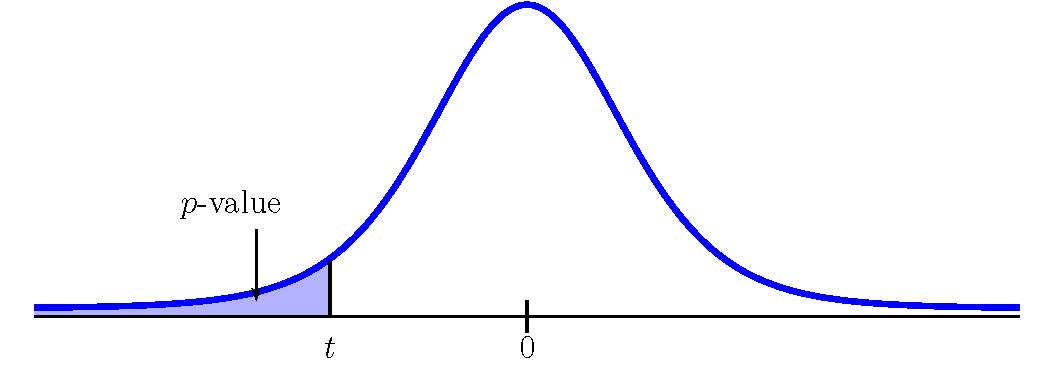
  If the p-value is the area in the left tail:

  • Use the t.dist function to find the p-value. In the t.dist(t-score, degrees of freedom, logic operator) function:
    • For t-score, enter the value of [latex]t[/latex] calculated from [latex]\displaystyle_1-\overline_2)-(\mu_1-\mu_2)>+\frac>>>[/latex].
    • For degrees of freedom, enter the degrees of freedom calculated using [latex]\displaystyle+\frac\right)^2>\times \left(\frac\right)^2+\frac\times \left(\frac\right)^2>>[/latex].
    • For the logic operator, enter true. Note: Because we are calculating the area under the curve, we always enter true for the logic operator.

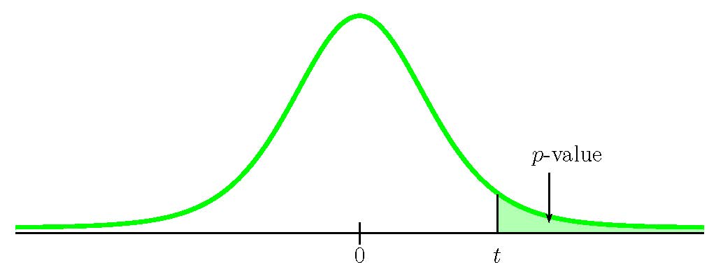
    If the p-value is the area in the right tail:

    • Use the t.dist.rt function to find the p-value. In the t.dist.rt(t-score, degrees of freedom) function:
      • For t-score, enter the value of [latex]t[/latex] calculated from [latex]\displaystyle_1-\overline_2)-(\mu_1-\mu_2)>+\frac>>>[/latex].
      • For degrees of freedom, enter the degrees of freedom calculated using [latex]\displaystyle+\frac\right)^2>\times \left(\frac\right)^2+\frac\times \left(\frac\right)^2>>[/latex].

      If the p-value is the sum of the area in the two tails:

      • Use the t.dist.2t function to find the p-value. In the t.dist.2t(t-score, degrees of freedom) function:
        • For t-score, enter the absolutevalue of [latex]t[/latex] calculated from [latex]\displaystyle_1-\overline_2)-(\mu_1-\mu_2)>+\frac>>>[/latex]. Note: In the t.dist.2t function, the value of the [latex]t[/latex]-score must be a positive number. If the [latex]t[/latex]-score is negative, enter the absolute value of the [latex]t[/latex]-score into the t.dist.2t function.
        • For degrees of freedom, enter the degrees of freedom calculated using [latex]\displaystyle+\frac\right)^2>\times \left(\frac\right)^2+\frac\times \left(\frac\right)^2>>[/latex].

        NOTE

        The degrees of freedom for a [latex]t[/latex]-distribution must be a whole number. The output from the degrees of freedom formula [latex]\displaystyle+\frac\right)^2> \times \left(\frac\right)^2+\frac \times \left(\frac\right)^2>>[/latex] is almost never a whole number. After calculating the value of [latex]df[/latex] using the formula, round the value down to the next whole number. Remember to entered the rounded down value of [latex]df[/latex] for the degrees of freedom in the t.dist functions.

        EXAMPLE

        A researcher wants to study the difference between the average amount of time boys and girls aged seven to eleven spend playing sports each day. In a sample of 9 girls, the average number of hours spent playing sports per day is 2 hours with a standard deviation of 0.866 hours. In a sample of 16 boys, the average number of hours spent playing sports per day is 3.2 hours with a standard deviation of 1 hours. Both populations have a normal distribution. At the 5% significance level, is there a difference in the mean amount of time boys and girls aged seven to eleven play sports each day?

        Solution:

        Let girls be population 1 and boys be population 2. These populations are independent because there is no relationship between the two groups. From the questions, we have the following information:

        Girls	Boys
        [latex]n_1=9[/latex]	[latex]n_2=16[/latex]
        [latex]\overline_1=2[/latex]	[latex]\overline_2=3.2[/latex]
        [latex]s=0.866[/latex]	[latex]s_2=1[/latex]

        Hypotheses:

        [latex]\begin H_0: & & \mu_1-\mu_2=0 \\ H_a: & & \mu_1-\mu_2 \neq 0 \end[/latex]

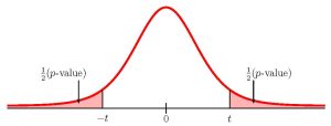
        This is a test on a the difference in two population means where the population standard deviation are unknown. So we use a [latex]t[/latex]-distribution to calculate the p-value. Because the alternative hypothesis is a [latex]\neq[/latex], the p-value is the sum of areas in the tails of the distribution.

        

        To use the t.dist.2t function, we need to calculate out the [latex]t[/latex]-score and the degrees of freedom:

        

        Function	t.dist.rt	Answer
        Field 1	0.8899…	0.1930
        Field 2	17

        So the p-value[latex]=0.1930[/latex].

        Conclusion:

        Because p-value[latex]=0.1930 \gt 0.01=\alpha[/latex], we do not reject the null hypothesis. At the 1% significance level there is not enough evidence to suggest that, on average, graduates of College A take more math classes than graduates of College B.

        NOTES

        1. The null hypothesis [latex]\mu_1-\mu_2=0[/latex] is the claim that the average number of math classes taken by graduates of College A equals the average number of math classes taken by graduates of College B. That is, the two populations have the same mean.
        2. The alternative hypothesis [latex]\mu_1 -\mu_2 \gt 0[/latex] is the claim that, on average, graduates of College A taken more math classes than graduates of College B ([latex]\mu_1 \gt \mu_2[/latex]).
        3. Keep all of the decimals throughout the calculation (i.e. in the [latex]t[/latex]-score, etc.) to avoid any round-off error in the calculation of the p-value. This ensures that we get the most accurate value for the p-value. Use Excel to do the calculations, and then click on the cells in subsequent calculations.
        4. The value of the degrees of freedom must be a whole number. After using the formula, remember to round the value down to the next whole number to get the required degrees of freedom for the [latex]t[/latex]-distribution.
        5. The p-value of 0.1930 is a large probability compared to the significance level, and so is likely to happen assuming the null hypothesis is true. This suggests that the assumption that the null hypothesis is true is most likely correct, and so the conclusion of the test is to not reject the null hypothesis. In other words, graduates from the two colleges take, on average, the same number of math classes.

        EXAMPLE

        A professor at a large community college taught both an online section and a face-to-face section of his statistics course. The professor wants to study the difference in the average score on the final exam, believing that the mean score for the online section would be lower than the face-to-face section. The professor randomly selected 30 final exam scores from each section and recorded the scores in the tables below.

        Online Section:

        67.6	41.2	85.3	55.9	82.4	91.2	73.5	94.1	64.7	64.7
        70.6	38.2	61.8	88.2	70.6	58.8	91.2	73.5	82.4	35.5
        94.1	88.2	64.7	55.9	88.2	97.1	85.3	61.8	79.4	79.4

        Face-to-Face Section:

        77.9	95.3	81.2	74.1	98.8	88.2	85.9	92.9	87.1	88.2
        69.4	57.6	69.4	67.1	97.6	85.9	88.2	91.8	78.8	71.8
        98.8	61.2	92.9	90.6	97.6	100	95.3	83.5	92.9	89.4

        At the 5% significance level, is the mean of the final exam score for the online section lower than the mean of the final exam score for the face-to-face section?

        Solution:

        Let the online section be population 1 and the face-to-face section be population 2. These populations are independent because there is no relationship between the two groups. From the questions, we have the following information:

        Online	Face-to-Face
        [latex]n_1=30[/latex]	[latex]n_2=30[/latex]
        [latex]\overline_1=72.85[/latex]	[latex]\overline_2=84.98[/latex]
        [latex]s_1=16.918. [/latex]	[latex]s_2=11.714. [/latex]

        Hypotheses:

        [latex]\begin H_0: & & \mu_1-\mu_2=0 \\ H_a: & & \mu_1-\mu_2 \lt 0 \end[/latex]

        This is a test on a the difference in two population means where the population standard deviation are unknown. So we use a [latex]t[/latex]-distribution to calculate the p-value. Because the alternative hypothesis is a [latex]\lt[/latex], the p-value is the area in the left tail of the distribution.

        

        To use the t.dist function, we need to calculate out the [latex]t[/latex]-score and the degrees of freedom:

        Function	t.dist	Answer
        Field 1	-3.228…	0.0011
        Field 2	51
        Field 3	true

        So the p-value[latex]=0.0011[/latex].

        Conclusion:

        Because p-value[latex]=0.0011 \lt 0.05=\alpha[/latex], we do reject the null hypothesis in favour of the alternative hypothesis. At the 5% significance level there is enough evidence to suggest that the mean final exam score for the online section is lower than the face-to-face section.

        NOTES

        1. The null hypothesis [latex]\mu_1-\mu_2=0[/latex] is the claim that the average final exam score is the same for both sections. That is, the two populations have the same mean.
        2. The alternative hypothesis [latex]\mu_1 -\mu_2 \lt 0[/latex] is the claim that average final exam score for the online section is lower than the face-to-face section ([latex]\mu_1 \lt \mu_2[/latex]).
        3. Keep all of the decimals throughout the calculation (i.e. in the sample means, sample standard deviations, in the [latex]t[/latex]-score, etc.) to avoid any round-off error in the calculation of the p-value. This ensures that we get the most accurate value for the p-value. Use Excel to do the calculations, and then click on the cells in subsequent calculations.
        4. The value of the degrees of freedom must be a whole number. After using the formula, remember to round the value down to the next whole number to get the required degrees of freedom for the [latex]t[/latex]-distribution.
        5. The p-value of 0.0011 is a small probability compared to the significance level, and so is unlikely to happen assuming the null hypothesis is true. This suggests that the assumption that the null hypothesis is true is most likely incorrect, and so the conclusion of the test is to reject the null hypothesis in favour of the alternative hypothesis. In other words, the average final exam score for the online section is lower than for the face-to-face section.

        TRY IT

        A study is done to determine if Company A retains its workers longer than Company B. Company A samples 15 workers, and their average time with the company is 5 years with a standard deviation of 1.2 years. Company B samples 20 workers, and their average time with the company is 4.5 years with a standard deviation of 0.8 years. The populations are normally distributed. At the 5% significance level, on average, do workers at Company A stay longer than workers at Company B?

        Click to see Solution

        Let Company A be population 1 and Company B be population 2.

        Hypotheses:

        [latex]\begin H_0: & & \mu_1-\mu_2=0 \\ H_a: & & \mu_1-\mu_2 \gt 0 \end[/latex]

        Function	t.dist.rt	Answer
        Field 1	1.3975…	0.0878
        Field 2	23

        Conclusion:

        Because p-value[latex]=0.0878 \gt 0.05=\alpha[/latex], we do not reject the null hypothesis. At the 5% significance level there is not enough evidence to suggest that, on average, workers at Company A stay longer than workers at Company B.

        Concept Review

        The general form of a confidence interval for the difference in two independent population means with unknown population standard deviations is

        where [latex]t[/latex] is the positive [latex]t[/latex]-score of the [latex]t[/latex]-distribution with [latex]\displaystyle+\frac\right)^2> \times \left(\frac\right)^2+\frac \times \left(\frac\right)^2>>[/latex] so that the area under the [latex]t[/latex]-distribution in between [latex]-t[/latex] and [latex]t[/latex] is [latex]C[/latex].

        The hypothesis test for the difference in two independent population means with unknown population standard deviations is a well established process:

        1. Write down the null and alternative hypotheses in terms of the differences in the population means [latex]\mu_1-\mu_2[/latex].
        2. Use the form of the alternative hypothesis to determine if the test is left-tailed, right-tailed, or two-tailed.
        3. Collect the sample information for the test and identify the significance level.
        4. Find the p-value (the area in the corresponding tail) for the test using the [latex]t[/latex]-distribution with [latex]\begin t & = & \frac<(\overline_1-\overline_2)-(\mu_1-\mu_2)>+\frac>> \\ \\ df & = & \frac<\left(\frac+\frac\right)^2>\times \left(\frac\right)^2+\frac\times \left(\frac\right)^2>\end[/latex] Because the population standard deviations are unknown, we use the [latex]t[/latex]-distribution to find the p-value.
        5. Compare the p-value to the significance level and state the outcome of the test.
        6. Write down a concluding sentence specific to the context of the question.